Basically many constraints have been developed in order to produce efficient search heuristics. Here we describe some popular methods which illustrate a broad range of heuristics.
The Oshima and Shirai Method (1979)
This method was one of the first methods developed to deal with a variety of classes of objects and to be able to recognise a scene described by depth maps containing multiple objects in any orientation. Objects are considered to have planar surfaces, smoothly curved surfaces or both. The classes of smoothly curved surfaces allowed include ellipsoids, hyperboloids, cones, paraboloids and cylinders.
This method operates in two stages.
The description is made using the segmentation of curved and planar surfaces from individual images. The segmentation method employed by Oshima and Shirai is a basic region growing method except that many surface properties and interrelationships are also calculated. These then are represented in a relational graph or semantic network. Typical surface properties for each region include:
The relationships between surfaces are characterised by:
Only a discrete set of views are used to model an object. Thus, for a complete model description of an object to be compiled, all unique views of the object must be presented to the system.
Fig. ![]() Oshima and Shirai matching method
The image data driven part of the search involves constructing one or more
kernels , each of which contains one or two regions that provide the
best potential matches to an object model. The chosen regions are selected according
to the criteria that they should, if possible, be planar, have large area, and have
many neighbours. The criteria are relaxed until ideally two regions or
at worst one region for the kernel is found.
Oshima and Shirai matching method
The image data driven part of the search involves constructing one or more
kernels , each of which contains one or two regions that provide the
best potential matches to an object model. The chosen regions are selected according
to the criteria that they should, if possible, be planar, have large area, and have
many neighbours. The criteria are relaxed until ideally two regions or
at worst one region for the kernel is found.
The model database is then searched for matches starting with the best kernel. If no match is found then another kernel is selected. If only one match is found using this kernel then the model driven matching phase is invoked. If more than one match is found then other possible kernels are also considered. The system suspends any further matching for kernels which give more than one match until all other kernels providing a single match have been considered by the model driven phase. Note that at the end of the matching process there could be more than one interpretation for a given kernel.
The model driven matching process of the second phase involves searching the scene around the kernel for regions corresponding to those in the model. The search is controlled by a similar type of depth first tree search that which we have already described.
At all stages regions are considered to be matched if a similarity function , based on region properties and relationships, is below a certain threshold.
When a match for a particular kernel has been found, a candidate body is said to have been found in the scene. The matching process continues until all scene regions have been tested for participating in a match. If only one candidate body is found in the scene then it is accepted as the desired match. Otherwise the scene requires further interpretation. If there are multiple candidates, they are examined to filter out inconsistent interpretations: two candidate bodies must be inconsistent if they share a region. For each kernel found a candidate body is rejected if one or more of its features are included in another candidate body which is consistent with respect to the same kernel. At the end of this process, hopefully one or perhaps more sets of mutually consistent interpretations will remain. Each such combination gives a possible interpretation of the scene from which position and orientation information can be calculated.
The 3DPO Method (1983)
The 3DPO (Three-dimensional Part Orientation) vision system was developed by Bolles and his colleagues to recognise and locate parts from depth maps for the purposes of directing a robot arm to grasp a wide range of moderately complex industrial parts. To achieve this goal they argued that most current vision strategies did not provide the required generality, being based upon simple generic object types such as polyhedra, cylinders, spheres or surface patches. Instead they adopted an entirely different approach that could recognise objects using only a few features or feature clusters that highly constrain the object (such as a circle with a fixed radius) and consequently the size of the solution search space. These ideas are now known as local feature focus methods.
The matching process consists of five stages:
This matching process uses an extended solid model. Here a form of boundary model) is augmented with a feature classification network. The feature network classifies features according to type and size, and groups features that share common surface normals, common axes (for cylinders) etc.
The ACRONYM Method (1979)
Brooks has developed a vision system, ACRONYM, that recognises three-dimensional objects occurring in two dimensional images. The examples given in the papers involve recognising airplanes on the runways of an airport from aerial photographs. He uses a generalised cylinder approach to represent both stored model and objects extracted from the image. . As in Nevatia and Binford's method (See next section), a relational graph structure is used to store the representation. Nodes are the generalised cylinders and the links represent the relative transformations (rotations and translations) between pairs of cylinders.
The system also uses two other graph structures, which are constructed from the object models, to help in the matching strategy:
Since the image is only two-dimensional account must be taken of the projection of the three-dimensional object features into two dimensions. Brooks uses two descriptions for two-dimensional features:
The matching process is performed in two stages:
This work has been extended by Kuan and Drazowich to permit use of three-dimensional images. The basic principles of ACRONYM are adhered to but surface properties are incorporated. Also, numerical feature measurements are used during matching (whereas there is a purely symbolic use of features in the original method). The surface properties are included in a multilevel representation of objects which is used in the prediction phase. The levels and the features represented at each level are:
The Grimson and Lozano-Perez Method (1984)
This method was originally designed to match sparse oriented surface points (points on an object with a surface normal attached) but has also been extended to match straight edges by Murray (1988) and others. Here we discuss the method in terms of matching straight line edges in a scene to straight line edges of a model, based on the work by Murray, as edges are more suitable than points when dense depth data is available. However, the discussion is equally valid for the case of oriented surface points. The only differences are that the points are matched to planar model faces and the implementation of some geometric constraints is slightly different.
The method requires the following assumptions:
This method is divided into two stages:
The two stages are now described separately.
Generating Feasible Interpretations
If an object model contains m edges and there are s sensed edges in the
scene then there are ![]() possible sets of complete interpretations which
match each sensed edge with some model edge. Only a few interpretations lead to
satisfactory solutions. Even for simple three-dimensional objects the number of
possible interpretations is very large. For example, a view of a cube can show up
to nine out of a possible twelve edges giving
possible sets of complete interpretations which
match each sensed edge with some model edge. Only a few interpretations lead to
satisfactory solutions. Even for simple three-dimensional objects the number of
possible interpretations is very large. For example, a view of a cube can show up
to nine out of a possible twelve edges giving ![]() possible
interpretations of which 24 are plausible. It should be noted that this number
can be very much larger greater still when sampled oriented points are employed
instead of edges. Clearly it is not possible to exhaustively test all these
interpretations for a match so the basic idea is to exploit some simple, local
geometric constraints on the sensed edges to minimise the number of interpretations
that must be tested explicitly.
possible
interpretations of which 24 are plausible. It should be noted that this number
can be very much larger greater still when sampled oriented points are employed
instead of edges. Clearly it is not possible to exhaustively test all these
interpretations for a match so the basic idea is to exploit some simple, local
geometric constraints on the sensed edges to minimise the number of interpretations
that must be tested explicitly.
The possible pairings of sensed and model edges are represented in the form of a search tree, called an interpretation tree.
At each level of the tree, one of the edges from the scene is matched with each of the m possible edges in the model. Each node has m children representing taking the match proposed so far together with all possible matches for the current scene edge. The result is a tree where complete paths to the deepest level correspond to complete matchings of object and scene edges. In the example shown in Fig. 55, we assume (unrealistically) for the purposes of illustration that the model has 4 edges and 3 edges have been found in the scene. Thus the pairings ((1,2),(2,1),(3,1)) corresponds to edge 1 in the scene matching edge 2 in the model, edge 2 in the scene matching edge 1 in the model and edge 3 in the scene matching edge 1 in the model. Note that because of errors in segmentation and other causes such as partial occlusion, it may be possible for more than one edge in the scene to correctly match a single edge in the model.
The interpretation tree is searched in depth first manner and pruned by rejecting interpretations that fail to meet one or more local geometric constraints. If the test is unsuccessful the current node and all of its descendants may be rejected as none of these descendants can possibly correct the current mismatch. In this way the potentially large search space is controlled.
The three local geometric constraints employed to prune the interpretation tree are:
The constraints used if matching oriented surface points to planar model faces are simpler:
An advantage of this constraint based approach is that all the model information required by the constraints can be computed off-line and stored in look up tables. Any information that is required for comparisons is then simply referred to as needed.
Model Testing
This second stage involves interrogating the sets of possible interpretations which are left after the first stage in order to firstly, estimate the transformation (rotation, scale and translation) between scene and model coordinates, and secondly, to check that all edges or surface points under the estimated transformation lie within acceptable bounds of the assigned edges or assigned faces.
The transformation is estimated by fitting the scene's description to the matched model edges. Two approaches can be applied to solve the problem. The first approach involves simply averaging the estimates of the transformation obtained for each matching pair. Details of the mathematics involved in this approach can be found in Grimson and Lozano-Perez's original paper or the Marshall and Martin Book. Alternatively, to produce more stable results, an approach similar to the estimation of rotation and translation presented in Marshall and Martin Book may be employed. This method is due to Faugeras and Hebert and has been employed by Murray and in the TINA vision system (discussed shortly).
Related Grimson and Lozano-Perez Methods
Apart from the Murray matching algorithm, several other approaches have been developed over recent years based on the Grimson and Lozano-Perez method. In particular Sheffield University's AI Vision Research Unit (AIVRU) have extended this strategy for their TINA vision system. This will be described in the next Section.
Lozano-Perez and Grimson have also developed their strategy to take into account overlapping and mismatching faces. This is achieved by incorporating an extra branch at each node in the interpretation tree to allow for null matches. This technique is described in detail later in Marshall and Martin Book as well as their papers..
Ikeuchi has developed a method for object manipulation tasks. He generates an interpretation tree from object views and then proceeds to orientate and locate objects in the scene using extended Gaussian images.
Recently, Brady and his colleagues have proposed a method of recognising objects
described by parameterised models. They aim to
allow recognition of objects that do not have or do not require explicit or fixed
representations. The example cited in the paper is that of a vision system mounted
on an autonomous guided vehicle navigating around a factory environment. This
system must recognise wooden pallets used for stacking. A pallet can have many
valid forms which humans readily recognise. However, a system using
fixed object models would only be able to recognise an observed pallet if it
were lucky enough to have a model of that particular pallet. To overcome this a
parameterised object model is used where each wooden slat's position ![]() relative to some reference point is allowed to vary in the
model, as shown in Fig. 57. The value of each
parameter
relative to some reference point is allowed to vary in the
model, as shown in Fig. 57. The value of each
parameter ![]() is determined in the matching process along with the rotation and
orientation.
is determined in the matching process along with the rotation and
orientation.
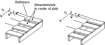
Fig. ![]() Parameterised representation of a pallet
The TINA Method
Parameterised representation of a pallet
The TINA Method
Sheffield University's AI Vision Research Unit (AIVRU) have developed a matching strategy for their TINA vision system. Much of their work has recently been published as a book containing a collection of papers related to the TINA vision system and other important aspects of three-dimensional model-based matching. Their method uses an approach similar to that of Grimson and Lozano-Perez except that the depth-first tree search is replaced by a hypothesise and test strategy. This grows feasible interpretations in order to improve the efficiency of the search. When some information in a scene may be missing (for example, when occlusion of an object occurs) tree searches tend to be combinatorially explosive. The hypothesise and test strategy is driven by selecting features from the image based on feature sizes and neighbourhoods. This hypothesise and test strategy is similar to the feature focus} methods used in the 3DPO matching algorithm discussed in for 3DPO.
The system matches three-dimensional edges (obtained by the use of passive stereo) to three-dimensional edge based models. The matching algorithm uses similar pairwise local geometric relationships to those of Grimson and Lozano-Perez and Murray to limit the search space further.
The basic method is as follows:
The Faugeras and Hebert Method (1983)
This method matches primitive surfaces extracted from a scene to ones in the model. In the original approach the method is described as coping with planar and quadric surfaces.
The basic approach is to try to match each primitive surface from the model, say
![]() , to one segmented from the scene,
, to one segmented from the scene, ![]() , to obtain a match pair
, to obtain a match pair ![]() . This is achieved using a tree search similar to the interpretation tree described
earlier. However, an estimation of the transformation (rotation and translation)
describing the mapping from model to scene is used as a constraint to control the
search as it proceeds, in contrast to the previous methods based on the Grimson and
Lozano-Perez method where the transformation is
only estimated after matching is completed.
. This is achieved using a tree search similar to the interpretation tree described
earlier. However, an estimation of the transformation (rotation and translation)
describing the mapping from model to scene is used as a constraint to control the
search as it proceeds, in contrast to the previous methods based on the Grimson and
Lozano-Perez method where the transformation is
only estimated after matching is completed.
From a small initial set of match pairs, the match list, an initial estimate of the transformation is made. Pairs of primitives from the scene and model are then added to this list if they are compatible with the match so far. Each time a successful match is found a new estimate of the transformation is calculated, and the process is continued until all scene primitives have been matched. If at any stage no possible match pair can be found then a backtracking mechanism is used. A match is considered to be successful if it is consistent with the existing transformation within an allowed tolerance.
Thus, the method exploits the global constraint of rigidity under the transformation to control the potentially combinatorially explosive search space. This is a major difference from the Grimson and Lozano-Perez method. The resulting paradigm of the Faugeras and Hebert method is that of recognising whilst locating, which is controlled mainly by global geometric constraints and not by testing a set of locally generated feasible interpretations. The use of global geometric constraints to control the search is generally more efficient.
At each step the estimation of the transformation is found by solving a least squares minimisation problem (not considered here -- details Marshall and Martin Book or original papers).
A cheap constraint is also employed at each level of the search in order to eliminate grossly mismatching pairs more quickly. The purpose of these tests is to provide a rough estimate of the geometric consistency of the new pair with the current match list. This test can be either or both of:
This method has been used in many different computer vision applications. It has been employed in matching in the two-dimensional domain, matching different depth maps and matching using simple occluding (or jump) edges and surface primitives. In the last case Hebert and Kanade argue that because segmentation of high order surface patches is unreliable, low level primitives should be used first to obtain a small number of possible solutions which are then tested using a detailed surface matcher. They employ simple occluding edges which are easily and reliably calculated to limit the number of possible interpretations.