A heuristic is a method that
The classic example of heuristic search methods is the travelling salesman problem.
Heuristic Search methods Generate and Test Algorithm
This method is basically a depth first search as complete solutions must be created before testing. It is often called the British Museum method as it is like looking for an exhibit at random. A heuristic is needed to sharpen up the search. Consider the problem of four 6-sided cubes, and each side of the cube is painted in one of four colours. The four cubes are placed next to one another and the problem lies in arranging them so that the four available colours are displayed whichever way the 4 cubes are viewed. The problem can only be solved if there are at least four sides coloured in each colour and the number of options tested can be reduced using heuristics if the most popular colour is hidden by the adjacent cube.
Hill climbing
Here the generate and test method is augmented by an heuristic function which measures the closeness of the current state to the goal state.
In the case of the four cubes a suitable heuristic is the sum of the number of different colours on each of the four sides, and the goal state is 16 four on each side. The set of rules is simply choose a cube and rotate the cube through 90 degrees. The starting arrangement can either be specified or is at random.
SIMULATED ANNEALING
This is a variation on hill climbing and the idea is to include a general survey of the scene to avoid climbing false foot hills.
The
whole space is explored initially and this avoids the danger of being caught on
a plateau or ridge and makes the procedure less sensitive to the starting
point. There are two additional changes; we go for minimisation rather than
creating maxima and we use the term objective function rather than heuristic.
It becomes clear that we are valley descending rather than hill climbing. The
title comes from the metallurgical process of heating metals and then letting
them cool until they reach a minimal energy steady final state. The probability
that the metal will jump to a higher energy level is given by
![]() where k is Boltzmann's constant. The rate at which
the system is cooled is called the annealing schedule.
where k is Boltzmann's constant. The rate at which
the system is cooled is called the annealing schedule. ![]() is called the
change in the value of the objective function and kT is called T a type of
temperature. An example of a problem suitable for such an algorithm is the
travelling salesman. The SIMULATED ANNEALING algorithm is based upon the
physical process which occurs in metallurgy where metals are heated to high
temperatures and are then cooled. The rate of cooling clearly affects the
finished product. If the rate of cooling is fast, such as when the metal is
quenched in a large tank of water the structure at high temperatures persists at
low temperature and large crystal structures exist, which in this case is
equivalent to a local maximum. On the other hand if the rate of cooling is slow
as in an air based method then a more uniform crystalline structure exists
equivalent to a global maximum.The probability of making a large uphill move is
lower than a small move and the probability of making large moves decreases with
temperature. Downward moves are allowed at any time.
is called the
change in the value of the objective function and kT is called T a type of
temperature. An example of a problem suitable for such an algorithm is the
travelling salesman. The SIMULATED ANNEALING algorithm is based upon the
physical process which occurs in metallurgy where metals are heated to high
temperatures and are then cooled. The rate of cooling clearly affects the
finished product. If the rate of cooling is fast, such as when the metal is
quenched in a large tank of water the structure at high temperatures persists at
low temperature and large crystal structures exist, which in this case is
equivalent to a local maximum. On the other hand if the rate of cooling is slow
as in an air based method then a more uniform crystalline structure exists
equivalent to a global maximum.The probability of making a large uphill move is
lower than a small move and the probability of making large moves decreases with
temperature. Downward moves are allowed at any time.
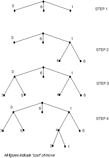
Best First Search
A combination of depth first and breadth first searches.
Depth first is good because a solution can be found without computing all nodes and breadth first is good because it does not get trapped in dead ends. The best first search allows us to switch between paths thus gaining the benefit of both approaches. At each step the most promising node is chosen. If one of the nodes chosen generates nodes that are less promising it is possible to choose another at the same level and in effect the search changes from depth to breadth. If on analysis these are no better then this previously unexpanded node and branch is not forgotten and the search method reverts to the descendants of the first choice and proceeds, backtracking as it were.
This process is very similar to steepest ascent, but in hill climbing once a move is chosen and the others rejected the others are never reconsidered whilst in best first they are saved to enable revisits if an impasse occurs on the apparent best path. Also the best available state is selected in best first even its value is worse than the value of the node just explored whereas in hill climbing the progress stops if there are no better successor nodes. The best first search algorithm will involve an OR graph which avoids the problem of node duplication and assumes that each node has a parent link to give the best node from which it came and a link to all its successors. In this way if a better node is found this path can be propagated down to the successors. This method of using an OR graph requires 2 lists of nodes
OPEN is a priority queue of nodes that have been evaluated by the heuristic function but which have not yet been expanded into successors. The most promising nodes are at the front. CLOSED are nodes that have already been generated and these nodes must be stored because a graph is being used in preference to a tree.
Heuristics In order to find the most promising nodes a heuristic function is needed called f' where f' is an approximation to f and is made up of two parts g and h' where g is the cost of going from the initial state to the current node; g is considered simply in this context to be the number of arcs traversed each of which is treated as being of unit weight. h' is an estimate of the initial cost of getting from the current node to the goal state. The function f' is the approximate value or estimate of getting from the initial state to the goal state. Both g and h' are positive valued variables. Best First The Best First algorithm is a simplified form of the A* algorithm. From A* we note that f' = g+h' where g is a measure of the time taken to go from the initial node to the current node and h' is an estimate of the time taken to solution from the current node. Thus f' is an estimate of how long it takes to go from the initial node to the solution. As an aid we take the time to go from one node to the next to be a constant at 1.
Best First Search Algorithm:
The A* Algorithm
Best first search is a simplified A*.
Graceful decay of admissibility
If h' rarely overestimates h by more than d then the A* algorithm will rarely find a solution whose cost is d greater than the optimal solution.