


| Frame | Original | Compressed | Error |
| 1 | |
|
|
| 2 | |
|
|
| 3 | |
|
|
| 4 | |
|
|
| 5 | |
|
|
| 6 | |
|
|
| 7 | |
|
|
| 8 | |
|
|
| 9 | |
|
|
| 10 | |
|
|
 Results:
Scale = 1 |
Scale = 8 |
Scale = 16 |
Scale = 32 |
Scale = 64 |
Scale = 112 |
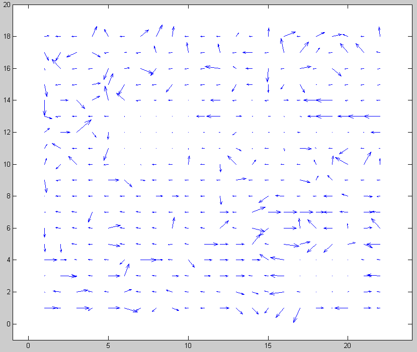 I tried reducing the beginning step size from 16 to 8 and that simple change corrected nearly all of the motion vectors. Now I realize that a step size of 16 is too large to do matching with a 16x16 macroblock. There is no overlap between the true macroblock location and the test areas. A video panning at about 8 pixels per frame would not correlate well with any of the test areas so an error is likely. Making an error in the first step of a logarithmic search significantly decreases the chances of finding a good motion vector.
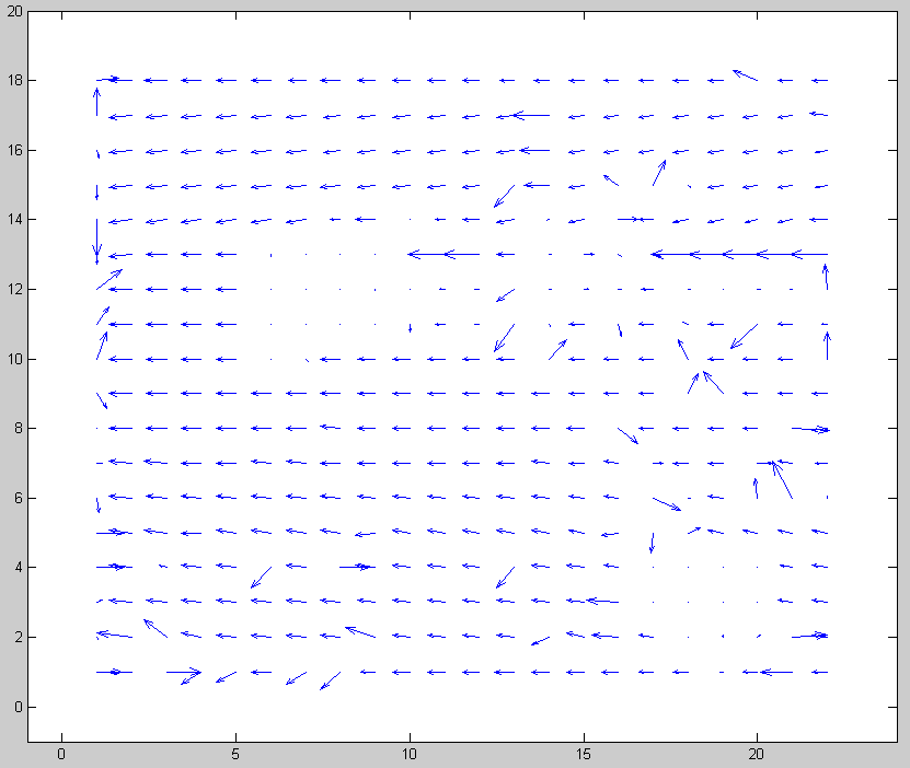
Below are the improved motion vectors for beginning step size = 8. Notice how consistent they are throughout the frame.
Step size = 8
I tried reducing the beginning step size from 16 to 8 and that simple change corrected nearly all of the motion vectors. Now I realize that a step size of 16 is too large to do matching with a 16x16 macroblock. There is no overlap between the true macroblock location and the test areas. A video panning at about 8 pixels per frame would not correlate well with any of the test areas so an error is likely. Making an error in the first step of a logarithmic search significantly decreases the chances of finding a good motion vector.
Below are the improved motion vectors for beginning step size = 8. Notice how consistent they are throughout the frame.
Step size = 8
 The really interesting point about this find is that a slower or faster panning video probably would not have shown this problem. It just happened that my test video panned at about 8 pixels per second, which is the worst case.
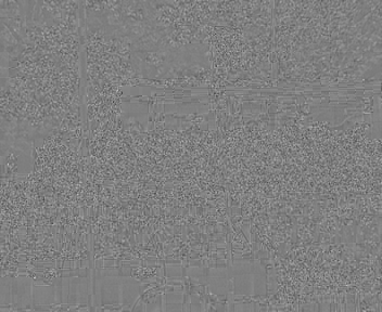
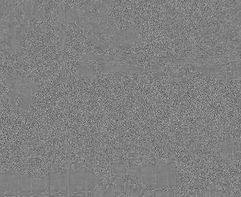
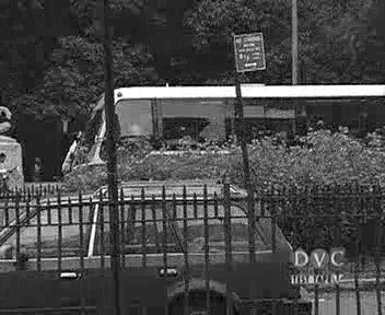
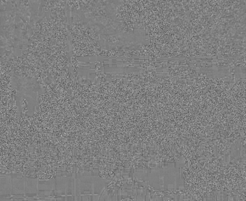
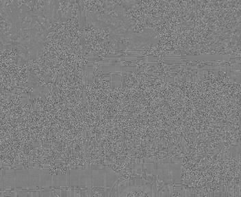
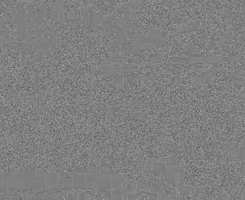
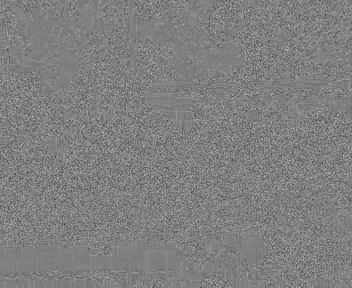
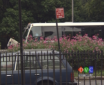
#### Reconstruction of a P frame without the residual
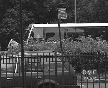
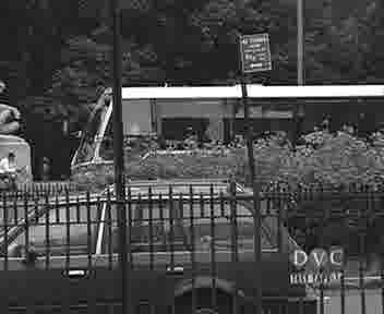
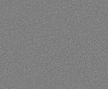
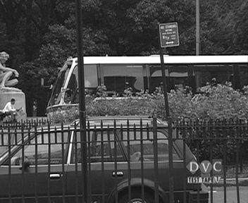
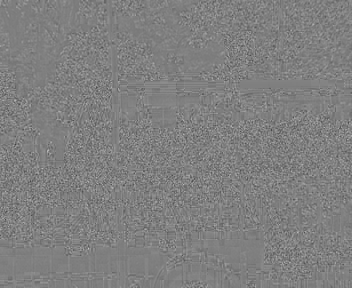
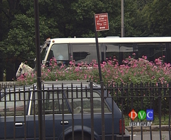
I was interested to see what kind of visual information gets encoded in the residual portion of a P frame and, conversely, how well a frame can be represented using just motion vectors. To see this, I encoded a P frame, then decoded it twice: once with the residual added, and once without.
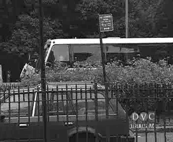
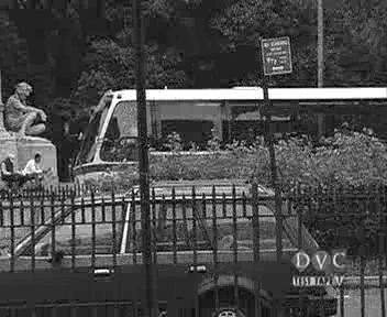
Original frame:
The really interesting point about this find is that a slower or faster panning video probably would not have shown this problem. It just happened that my test video panned at about 8 pixels per second, which is the worst case.
#### Reconstruction of a P frame without the residual
I was interested to see what kind of visual information gets encoded in the residual portion of a P frame and, conversely, how well a frame can be represented using just motion vectors. To see this, I encoded a P frame, then decoded it twice: once with the residual added, and once without.
Original frame:
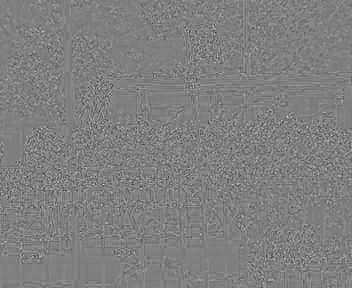
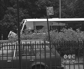
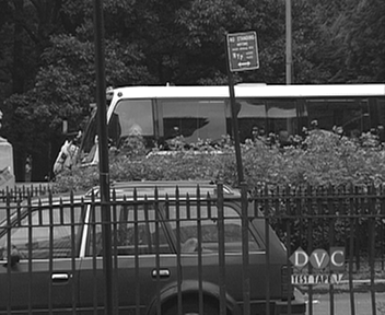
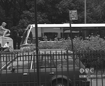
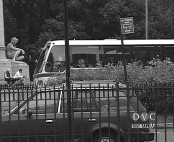
Decoded with residual: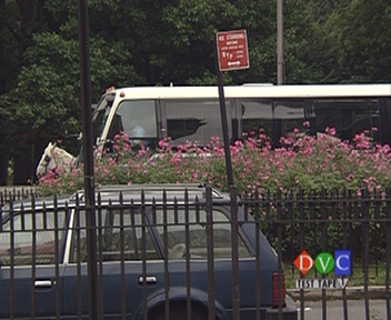 |
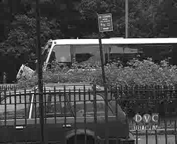
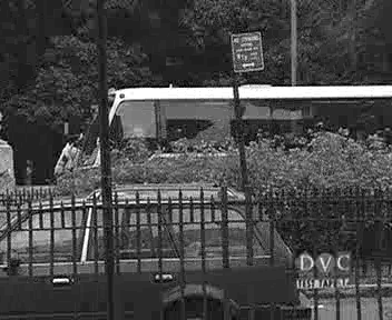
Decoded without residual: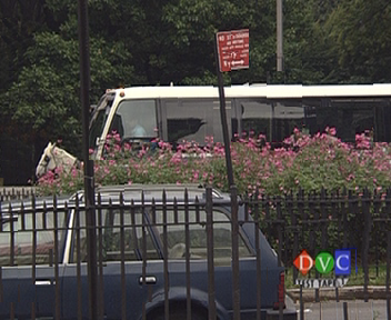 |
| Frame type | Encode time (sec/frame) | Decode time (sec/frame) |
| I | 2.1 | 1.3 |
| P | 1.8 | 1.3 |
| Search type | Encode time (sec/frame) | Decode time (sec/frame) |
| Sequential | 9.0 | 1.3 |
| Logarithmic | 1.8 | 1.3 |